Pytorch与视觉竞赛入门1-网络层原理和使用

Pytorch全连接层原理和使用

矩阵乘法实现全连接层

方法1：矩阵乘法

x = torch.arange(0, 100, 0.01,dtype=torch.float32)
y = (10 * x + 5 + np.random.normal(0, 1, x.size())).float()

batch_size = 100
w = torch.randn((1,), requires_grad=True,dtype=torch.float32)
b = torch.randn((1,), requires_grad=True,dtype=torch.float32)

loss = nn.MSELoss()
iter_time = x.size()[0]//batch_size
optimizer = torch.optim.Adam([w,b], lr=0.1,weight_decay=0.1)

for e in range(5):
    for t in range(iter_time):
        train_x=x[batch_size*t:batch_size*(t+1)].clone()
        train_y = y[batch_size * t:batch_size * (t + 1)].clone()
        z = torch.einsum('i,j->ij',train_x,w)+b #z=w*x+b
        
        output = loss(train_y,z)
        optimizer.zero_grad()
        output.backward() #通过loss反向传播
        optimizer.step()
        print(e,t,output/batch_size)
#w=9.9682
#b=8.1066

方法2：利用nn.Parameters()

模型中可学习的参数由nn.Parameters()注册到模型中。

class Linear(nn.Module):
    def __init__(self, in_features: int, out_features: int, bias: bool = True) -> None:
        super(Linear, self).__init__()
        self.in_features = in_features
        self.out_features = out_features
        self.weight = nn.Parameter(torch.Tensor(out_features, in_features))
        if bias:
        	self.bias = nn.Parameter(torch.Tensor(out_features))
        else:
            self.register_parameter('bias', None)
        self.reset_parameters()
    def reset_parameters(self) -> None:
        nn.init.kaiming_uniform_(self.weight, a=np.sqrt(5))
        if self.bias is not None:
            fan_in, _ = nn.init._calculate_fan_in_and_fan_out(self.weight)
            bound = 1 / np.sqrt(fan_in)
            nn.init.uniform_(self.bias, -bound, bound)

    def forward(self, input: torch.Tensor) -> torch.Tensor:
        output = input.matmul(self.weight.t())
        if self.bias is not None:
            output += self.bias
        return output
linear= Linear(1,1)
num_epochs = 5
criterion = nn.MSELoss()
optimizer = torch.optim.Adam(linear.parameters(), lr=0.1,weight_decay=0.1)

for epoch in range(num_epochs):
    for t in range(iter_time):
        train_x=x[batch_size*t:batch_size*(t+1)].clone()
        train_y = y[batch_size * t:batch_size * (t + 1)].clone()
        train_x=train_x.unsqueeze(1)
        train_y=train_y.unsqueeze(1)
        # forward
        out = linear(train_x) # 前向传播
        loss = criterion(out, train_y) # 计算loss
        # backward
        optimizer.zero_grad() # 梯度归零
        loss.backward() # 方向传播
        optimizer.step() # 更新参数

        if (t+1) % 20 == 0:
            print('Epoch[{}/{}], loss: {:.6f}'.format(epoch+1,t,loss.data))
#w=9.9577
#b=9.0406

使用nn.Linear层

import torch.nn as nn
import torch.nn.functional as F

class Net(nn.Module):
    def __init__(self):
        super(Net, self).__init__()
        self.fc1   = nn.Linear(1, 1) # an affine operation: y = Wx + b
    def forward(self, x):
        x=self.fc1(x)
        return x
net = Net()
net

'''神经网络的结构是这样的
Net (
  (fc1): Linear (1 -> 1)
)
'''
num_epochs = 5
criterion = nn.MSELoss()
optimizer = torch.optim.Adam(net.parameters(), lr=0.05,weight_decay=0.1)
for epoch in range(num_epochs):
    for t in range(iter_time):
        train_x=x[batch_size*t:batch_size*(t+1)].clone()
        train_y = y[batch_size * t:batch_size * (t + 1)].clone()
        train_x=train_x.unsqueeze(1)
        train_y=train_y.unsqueeze(1)
        inputs = Variable(train_x)
        target = Variable(train_y)

        # forward
        out = net(inputs) # 前向传播
        loss = criterion(out, target) # 计算loss
        # backward
        optimizer.zero_grad() # 梯度归零
        loss.backward() # 方向传播
        optimizer.step() # 更新参数

        if (t+1) % 20 == 0:
            print('Epoch[{}/{}], loss: {:.6f}'.format(epoch+1,t+1,loss.data))
#w=9.9515
#b=8.6728

PyTorch卷积层原理和使用

参考资料：

如何理解空洞卷积（dilated convolution）？ - 谭旭的回答 - 知乎

如何理解空洞卷积（dilated convolution）？ - 刘诗昆的回答 - 知乎

Pytorch之卷积层

卷积尺寸计算

不考虑空洞卷积，假设输入图片大小为 $ I I$，卷积核大小为 $k \times k$，stride 为 $s$，padding 的像素数为 $p$，图片经过卷积之后的尺寸 $ O $ 如下： \[ O = \displaystyle\frac{I -k + 2 \times p}{s} +1 \]

Standard Convolution with a 3 x 3 kernel (and padding)

若考虑空洞卷积，假设输入图片大小为 $ I I$，卷积核大小为 $k \times k$，stride 为 $s$，padding 的像素数为 $p$，dilation 为 $d$，图片经过卷积之后的尺寸 $ O $ 如下： \[ O = \displaystyle\frac{I - d \times (k-1) + 2 \times p -1}{s} +1 \]

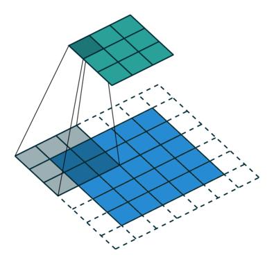
Dilated Convolution with a 3 x 3 kernel and dilation rate 2

小练习

如下卷积层的参数量是多少？

若将batch_size=16，64*64大小的RGB图片输入该卷积层，输出张量的形状为？

nn.Conv2d(
            in_channels=3,
            out_channels=32,
            kernel_size=5,
            stride=1,
            padding=2
            )

参数量为： \[ \begin {align}参数量&=in\_channels \times out\_channels \times kernel\_size+batch\_size \\&=3 \times 32 \times 5 \times 5+16 \\&=2416 \end {align} \] 图片大小为64*64，RGB表示channels数为3，根据公式： \[ O = \displaystyle\frac{64 -5 + 2 \times 2}{1} +1=64 \] 则输出张量形状为：batch_size=16, 64*64*32。

空洞卷积

图像分割FCN中有两个关键，一个是pooling减小图像尺寸增大感受野，另一个是upsampling扩大图像尺寸。在先减小再增大尺寸的过程中，肯定有一些信息损失掉了，那么能不能设计一种新的操作，不通过pooling也能有较大的感受野看到更多的信息呢？答案就是dilated conv。

dilated conv不是在像素之间padding空白的像素，而是在已有的像素上，skip掉一些像素，或者输入不变，对conv的kernel参数中插一些0的weight，达到一次卷积看到的空间范围变大的目的。

将普通的卷积stride步长设为大于1，也会达到增加感受野的效果，但是stride大于1就会导致downsampling，图像尺寸变小。

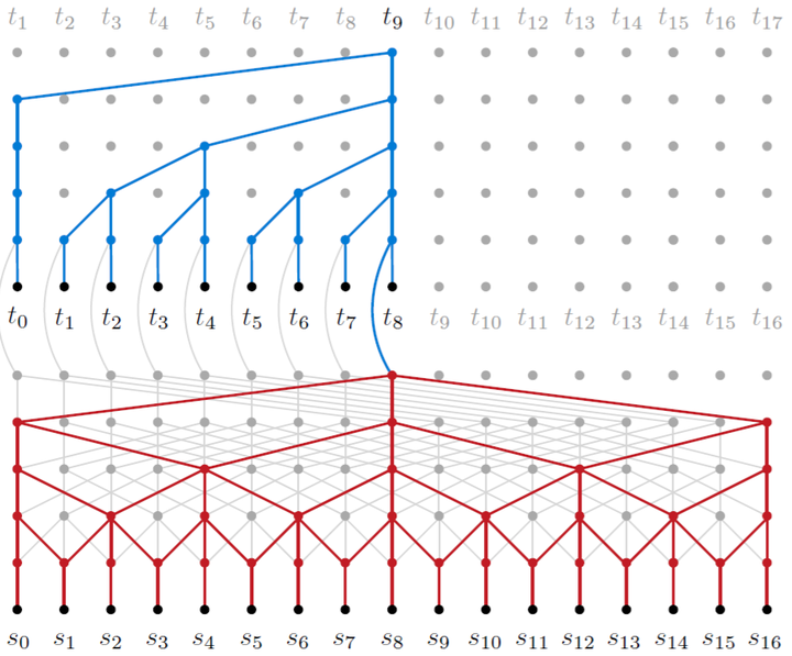
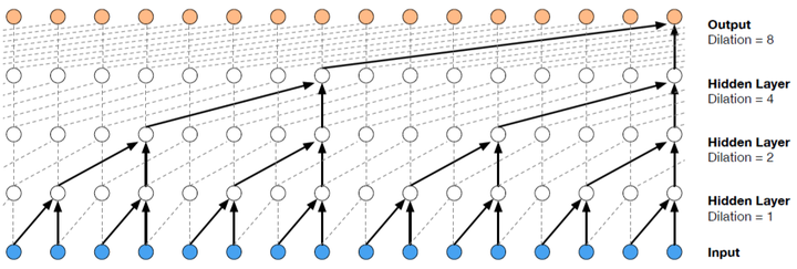
dilated的好处是不做pooling损失信息的情况下，加大了感受野，让每个卷积输出都包含较大范围的信息。在图像需要全局信息或者语音文本需要较长的sequence信息依赖的问题中，都能很好的应用dilated conv，比如图像分割[3]、语音合成WaveNet[2]、机器翻译ByteNet[1]中。简单贴下ByteNet和WaveNet用到的dilated conv结构，可以更形象的了解dilated conv本身。

ByteNet

WaveNet

torch.nn中的卷积层

torch.nn.Conv_N_d参数

class torch.nn.Conv1d(in_channels, out_channels, kernel_size, stride=1, padding=0, dilation=1, groups=1, bias=True)

class torch.nn.Conv2d(in_channels, out_channels, kernel_size, stride=1, padding=0, dilation=1, groups=1, bias=True)

class torch.nn.Conv3d(in_channels, out_channels, kernel_size, stride=1, padding=0, dilation=1, groups=1, bias=True)

in_channels(int) – 输入信号的通道   
out_channels(int) – 卷积产生的通道
kerner_size(int or tuple) - 卷积核的尺寸
stride(int or tuple, optional) - 卷积步长
padding (int or tuple, optional)- 输入的每一条边补充0的层数   
dilation(int or tuple, optional) – 卷积核元素之间的间距
groups(int, optional) – 从输入通道到输出通道的阻塞连接数
bias(bool, optional) - 如果bias=True，添加偏置

一维卷积

定义及输入输出

class torch.nn.Conv1d(in_channels, out_channels, kernel_size, stride=1, padding=0, dilation=1, groups=1, bias=True) input: (N,C_in,L_in) N为批次，C_in即为in_channels，即一批内输入一维数据个数，L_in是是一维数据基数 output: (N,C_out,L_out) N为批次，C_in即为out_channels，即一批内输出一维数据个数，L_out是一维数据基数

实操

conv1 = nn.Conv1d( 
            in_channels=5,
            out_channels=32,
            kernel_size=5,
            stride=1,
            padding=2  #padding是需要计算的，padding=（stride-1）/2
)
#只能接受tensor/variable
conv1(torch.Tensor(16, 5, 3))
conv1(Variable(torch.Tensor(16, 5, 3)))

二维卷积

class torch.nn.Conv2d(in_channels, out_channels, kernel_size, stride=1, padding=0, dilation=1, groups=1, bias=True)

input: (N,C_in,H_in,W_in) N为批次，C_in即为in_channels，即一批内输入二维数据个数，H_in是二维数据行数，W_in是二维数据的列数 output: (N,C_out,H_out,W_out) N为批次，C_out即为out_channels，即一批内输出二维数据个数，H_out是二维数据行数，W_out是二维数据的列数

实操

conv2 = nn.Conv2d( 
            in_channels=5,
            out_channels=32,
            kernel_size=5,
            stride=1,
            padding=2  #padding是需要计算的，padding=（stride-1）/2
)
#只能接受tensor/variable
conv2(torch.Tensor(16, 5, 3, 10))
conv2(Variable(torch.Tensor(16, 5, 3, 10)))

三维卷积

class torch.nn.Conv3d(in_channels, out_channels, kernel_size, stride=1, padding=0, dilation=1, groups=1, bias=True)

input: (N,C_in,D_in,H_in,W_in) output: (N,C_out,D_out,H_out,W_out)

实操

conv3 = nn.Conv3d( 
            in_channels=5,
            out_channels=32,
            kernel_size=5,
            stride=1,
            padding=2  #padding是需要计算的，padding=（stride-1）/2
)
#只能接受tensor/variable
conv3(torch.Tensor(16, 5, 3, 10, 12))
conv3(Variable(torch.Tensor(16, 5, 3, 10, 12)))

torch.nn.functional中的卷积函数

和torch.nn下的卷积层的区别在于，torch.nn.functional下的是函数，不是实际的卷积层，而是有卷积层功能的卷积层函数，所以它并不会出现在网络的图结构中。

torch.nn.functional.conv_N_d参数

weight：过滤器的形状 (out_channels, in_channels, kW)
bias：可选偏置的形状 (out_channels)
stride：卷积核的步长，默认为1

一维卷积

torch.nn.functional.conv1d(input, weight, bias=None, stride=1, padding=0, dilation=1, groups=1) input: (N,C_in,L_in) N为批次，C_in即为in_channels，即一批内输入一维数据个数，L_in是是一维数据基数 output: (N,C_out,L_out) N为批次，C_in即为out_channels，即一批内输出一维数据个数，L_out是一维数据基数

实操

filters = autograd.Variable(torch.randn(33, 16, 3))
inputs = autograd.Variable(torch.randn(20, 16, 50))
F.conv1d(inputs, filters)

二维卷积

torch.nn.functional.conv2d(input, weight, bias=None, stride=1, padding=0, dilation=1, groups=1)

实操

# With square kernels and equal stride
filters = autograd.Variable(torch.randn(8,4,3,3))
inputs = autograd.Variable(torch.randn(1,4,5,5))
F.conv2d(inputs, filters, padding=1)

三维卷积

torch.nn.functional.conv3d(input, weight, bias=None, stride=1, padding=0, dilation=1, groups=1)

input: (N,C_in,D_in,H_in,W_in) output: (N,C_out,D_out,H_out,W_out)

实操

filters = autograd.Variable(torch.randn(33, 16, 3, 3, 3))
inputs = autograd.Variable(torch.randn(20, 16, 50, 10, 20))
F.conv3d(inputs, filters)

PyTorch池化/反池化层和归一化层

池化层pooling layer

可参考官方文档：Pooling layers

池化层的作用：(1) 降低信息冗余；(2) 提升模型的尺度不变性、旋转不变性；(3) 防止过拟合。

池化层的常见操作包含以下几种：最大值池化，均值池化，随机池化，中值池化，组合池化等。

最大池化max pooling

在前向过程，选择图像区域中的最大值作为该区域池化后的值；在后向过程中，梯度通过前向过程时的最大值反向传播，其他位置的梯度为0.

在实际应用时，最大值池化又分为：重叠池化与非重叠池化。如AlexNet/GoogLeNet系列中采用的重叠池化，VGG中采用的非重叠池化。但是，自ResNet之后，池化层在分类网络中应用逐渐变少，往往采用stride=2的卷积替代最大值池化层。

最大值池化的优点在于它能学习到图像的边缘和纹理结构。

参数：

kernel_size- 窗口大小
stride- 步长。默认值是kernel_size
padding - 补0数
dilation– 控制窗口中元素步幅的参数
return_indices - 如果等于True，会返回输出最大值的序号，对于上采样操作会有帮助
ceil_mode - 如果等于True，计算输出信号大小的时候，会使用向上取整，代替默认的向下取的操作

torch.nn.MaxPool1d(kernel_size, stride=None, padding=0, dilation=1, return_indices=False, ceil_mode=False)
torch.nn.MaxPool2d(kernel_size, stride=None, padding=0, dilation=1, return_indices=False, ceil_mode=False)
torch.nn.MaxPool3d(kernel_size, stride=None, padding=0, dilation=1, return_indices=False, ceil_mode=False)

torch.nn.MaxPool_N_d实操

max1=torch.nn.MaxPool1d(3,1,0,1)
max1(torch.Tensor(16,15,15))
#output_shape=torch.Size([16, 15, 13])

max2=torch.nn.MaxPool2d(3,1,0,1)
max2(torch.Tensor(16,15,15,14))
#output_shape=torch.Size([16, 15, 13, 12])

max3=torch.nn.MaxPool3d(3,1,0,1)
max3(torch.Tensor(16,15,15,12,20))
#output_shape=torch.Size([16, 15, 13, 10, 18])

均值池化mean/average pooling

参数：

kernel_size - 池化窗口大小
stride- 步长。默认值是kernel_size
padding- 输入的每一条边补充0的层数
dilation – 一个控制窗口中元素步幅的参数
return_indices - 如果等于True，会返回输出最大值的序号，对于上采样操作会有帮助
ceil_mode - 如果等于True，计算输出信号大小的时候，会使用向上取整，代替默认的向下取整的操作

torch.nn.AvgPool1d(kernel_size, stride=None, padding=0, ceil_mode=False, count_include_pad=True)
torch.nn.AvgPool2d(kernel_size, stride=None, padding=0, ceil_mode=False, count_include_pad=True)
torch.nn.AvgPool3d(kernel_size, stride=None, padding=0, ceil_mode=False, count_include_pad=True)

torch.nn.AvgPool_N_d实操

类似torch.nn.MaxPool_N_d

反池化层

是池化的一个“逆”过程，但“逆”只是通过上采样恢复到原来的尺寸，像素值是不能恢复成原来一模一样，因为像最大池化是不可逆的，除最大值之外的像素都已经丢弃了。

最大值反池化nn.MaxUnpool2d

功能：对二维图像进行最大值池化上采样

参数：

kernel_size- 窗口大小
stride - 步长。默认值是kernel_size
padding - 补0数

torch.nn.MaxUnpool1d(kernel_size, stride=None, padding=0)
torch.nn.MaxUnpool2d(kernel_size, stride=None, padding=0)
torch.nn.MaxUnpool3d(kernel_size, stride=None, padding=0)

torch.nn.MaxPool2d实操

img_tensor=torch.Tensor(16,5,32,32)
# 上采样
max_pool = nn.MaxPool2d(kernel_size=(2, 2), stride=(2, 2), return_indices=True, ceil_mode=True)
img_pool, indices = max_pool(img_tensor)
 
# 下采样
img_unpool = torch.rand_like(img_pool, dtype=torch.float)   # 输入图像的大小和上采样的大小保持一致
max_unpool = nn.MaxUnpool2d((2, 2), stride=(2, 2))   
img_unpool = max_unpool(img_unpool, indices)

组合池化

组合池化同时利用最大值池化与均值池化两种的优势而引申的一种池化策略。常见组合策略有两种：Cat与Add。其代码描述如下：

def add_avgmax_pool2d(x, output_size=1):
    x_avg = F.adaptive_avg_pool2d(x, output_size)
    x_max = F.adaptive_max_pool2d(x, output_size)
    return 0.5 * (x_avg + x_max)

def cat_avgmax_pool2d(x, output_size=1):
    x_avg = F.adaptive_avg_pool2d(x, output_size)
    x_max = F.adaptive_max_pool2d(x, output_size)
    return torch.cat([x_avg, x_max], 1)

归一化层normalization layer

可以参考之前的博客：Transformer相关——（6）Normalization方式 | 冬于的博客 (ifwind.github.io)

官方文档：Normalization Layers

BatchNorm

torch.nn.BatchNorm1d(num_features, eps=1e-05, momentum=0.1, affine=True, track_running_stats=True)
torch.nn.BatchNorm2d(num_features, eps=1e-05, momentum=0.1, affine=True, track_running_stats=True)
torch.nn.BatchNorm3d(num_features, eps=1e-05, momentum=0.1, affine=True, track_running_stats=True)

参数：

num_features： 来自期望输入的特征数，该期望输入的大小为batch_size × num_features [× width]，和之前输入卷积层的channel位的维度数目相同
eps： 为保证数值稳定性（分母不能趋近或取0）,给分母加上的值。默认为1e-5。
momentum： 动态均值和动态方差所使用的动量。默认为0.1。
affine： 布尔值，当设为true，给该层添加可学习的仿射变换参数。
track_running_stats：布尔值，当设为true，记录训练过程中的均值和方差；

# With Learnable Parameters
m = nn.BatchNorm2d(5)
# Without Learnable Parameters
m = nn.BatchNorm2d(5, affine=False)
inputs = torch.randn(20, 5, 35, 45)
output = m(inputs)

LayerNorm

torch.nn.LayerNorm(normalized_shape, eps=1e-05, elementwise_affine=True)

参数：

normalized_shape： 输入尺寸
[× normalized_shape[0] × normalized_shape[1]×…× normalized_shape[−1]]
eps： 为保证数值稳定性（分母不能趋近或取0）,给分母加上的值。默认为1e-5。
elementwise_affine： 布尔值，当设为true，给该层添加可学习的仿射变换参数。

LayerNorm就是对(2, 2,4), 后面这一部分进行整个的标准化。可以理解为对整个图像进行标准化。

x_test = np.array([[[1,2,-1,1],[3,4,-2,2]],
                   [[1,2,-1,1],[3,4,-2,2]]])
x_test = torch.from_numpy(x_test).float()

m = nn.LayerNorm(normalized_shape = [2,4])
output = m(x_test)

InstanceNorm

torch.nn.InstanceNorm1d(num_features, eps=1e-05, momentum=0.1, affine=False, track_running_stats=False)
torch.nn.InstanceNorm2d(num_features, eps=1e-05, momentum=0.1, affine=False, track_running_stats=False)
torch.nn.InstanceNorm3d(num_features, eps=1e-05, momentum=0.1, affine=False, track_running_stats=False)

参数：

num_features： 来自期望输入的特征数，该期望输入的大小为batch_size x num_features [x width]
eps： 为保证数值稳定性（分母不能趋近或取0）,给分母加上的值。默认为1e-5。
momentum： 动态均值和动态方差所使用的动量。默认为0.1。
affine： 布尔值，当设为true，给该层添加可学习的仿射变换参数。
track_running_stats：布尔值，当设为true，记录训练过程中的均值和方差；

InstanceNorm就是对(2, 2, 4)最后这一部分进行Norm。

x_test = np.array([[[1,2,-1,1],[3,4,-2,2]],
                   [[1,2,-1,1],[3,4,-2,2]]])
x_test = torch.from_numpy(x_test).float()

m = nn.InstanceNorm1d(num_features=2)
output = m(x_test)

GroupNorm

torch.nn.GroupNorm(num_groups, num_channels, eps=1e-05, affine=True)

参数：

num_groups：需要划分为的groups
num_features： 来自期望输入的特征数，该期望输入的大小为batch_size x num_features [x width]
eps： 为保证数值稳定性（分母不能趋近或取0）,给分母加上的值。默认为1e-5。
momentum： 动态均值和动态方差所使用的动量。默认为0.1。
affine： 布尔值，当设为true，给该层添加可学习的仿射变换参数。

当GroupNorm中group的数量是1的时候, 是与上面的LayerNorm是等价的。

x_test = np.array([[[1,2,-1,1],[3,4,-2,2]],
                   [[1,2,-1,1],[3,4,-2,2]]])
x_test = torch.from_numpy(x_test).float()
# Separate 2 channels into 1 groups (equivalent with LayerNorm)
m = nn.GroupNorm(num_groups=1, num_channels=2, affine=False)
output = m(x_test)

当GroupNorm中num_groups的数量等于num_channel的数量，与InstanceNorm等价。

# Separate 2 channels into 2 groups (equivalent with InstanceNorm)
m = nn.GroupNorm(num_groups=2, num_channels=2, affine=False)
output = m(x_test)

参考资料

如何理解空洞卷积（dilated convolution）？ - 谭旭的回答 - 知乎

如何理解空洞卷积（dilated convolution）？ - 刘诗昆的回答 - 知乎

Pytorch之卷积层

Pytorch MaxUnpooling 反最大池化操作(上采样)

PyTorch快速入门教程二（线性回归以及logistic回归）

Pytorch全连接网络