Pytorch与深度学习自查手册3-模型定义

定义神经网络

继承nn.Module类；
初始化函数__init__：网络层设计；
forward函数：模型运行逻辑。

class NeuralNetwork(nn.Module):
    def __init__(self):
        super(NeuralNetwork, self).__init__()
        self.flatten = nn.Flatten()
        self.linear_relu_stack = nn.Sequential(
            nn.Linear(28*28, 512),
            nn.ReLU(),
            nn.Linear(512, 512),
            nn.ReLU(),
            nn.Linear(512, 10),
        )

    def forward(self, x):
        x = self.flatten(x)
        logits = self.linear_relu_stack(x)
        return logits

权重初始化

pytorch中的权值初始化

方法1：net.apply(weights_init)

def weights_init(m):
    classname = m.__class__.__name__
    if classname.find('Conv') != -1:
        nn.init.normal_(m.weight.data, 0.0, 0.02)
    elif classname.find('BatchNorm') != -1:
        nn.init.normal_(m.weight.data, 1.0, 0.02)
        nn.init.constant_(m.bias.data, 0)

net=Model()
net.apply(weights_init)

方法2：在网络初始化的时候进行参数初始化

使用net.modules()遍历模型中的网络层的类型；
对其中的m层的weigth.data(tensor)部分进行初始化操作。

class Model(nn.Module):
    def __init__(self, block, layers, num_classes=1000):
        self.inplanes = 64
        super(Model, self).__init__()
        self.conv1 = nn.Conv2d(3, 64, kernel_size=7, stride=2, padding=3,
                               bias=False)
        self.bn1 = nn.BatchNorm2d(64)
        self.relu = nn.ReLU(inplace=True)
        self.maxpool = nn.MaxPool2d(kernel_size=3, stride=2, padding=1)
        self.layer1 = ...
        ...
        #　权值参数初始化
        for m in self.modules():
            if isinstance(m, nn.Conv2d):
                n = m.kernel_size[0] * m.kernel_size[1] * m.out_channels
                m.weight.data.normal_(0, math.sqrt(2. / n))
            elif isinstance(m, nn.BatchNorm2d):
                m.weight.data.fill_(1)
                m.bias.data.zero_()

常用的操作

利用nn.Parameter()设计新的层

import torch
from torch import nn

class MyLinear(nn.Module):
  def __init__(self, in_features, out_features):
    super().__init__()
    self.weight = nn.Parameter(torch.randn(in_features, out_features))
    self.bias = nn.Parameter(torch.randn(out_features))

  def forward(self, input):
    return (input @ self.weight) + self.bias

nn.Flatten

展平输入的张量： 28x28 -> 784

input = torch.randn(32, 1, 5, 5)
m = nn.Sequential(
    nn.Conv2d(1, 32, 5, 1, 1),
    nn.Flatten()
)
output = m(input)
output.size()

nn.Sequential

一个有序的容器，神经网络模块将按照在传入构造器的顺序依次被添加到计算图中执行，同时以神经网络模块为元素的有序字典也可以作为传入参数。

net = nn.Sequential(
   ('fc1',MyLinear(4, 3)),
   ('act',nn.ReLU()),
   ('fc2',MyLinear(3, 1))
)

常用的层

全连接层nn.Linear()

torch.nn.Linear(in_features, out_features, bias=True,device=None, dtype=None)

in_features: 输入维度
out_features:输出维度
bias: 是否有偏置

m = nn.Linear(20, 30)
input = torch.randn(128, 20)
output = m(input)
print(output.size())

torch.nn.Dropout

'''
p：将元素置0的概率，默认值=0.5
'''
torch.nn.Dropout(p=0.5, inplace=False)

卷积`torch.nn.ConvNd()`

class torch.nn.Conv2d(in_channels, out_channels, kernel_size, stride=1, padding=0, dilation=1, groups=1, bias=True)

in_channels(int) – 输入信号的通道   
out_channels(int) – 卷积产生的通道
kerner_size(int or tuple) - 卷积核的尺寸
stride(int or tuple, optional) - 卷积步长
padding (int or tuple, optional)- 输入的每一条边补充0的层数   
dilation(int or tuple, optional) – 卷积核元素之间的间距
groups(int, optional) – 从输入通道到输出通道的阻塞连接数
bias(bool, optional) - 如果bias=True，添加偏置

input: (N,C_in,H_in,W_in) N为批次，C_in即为in_channels，即一批内输入二维数据个数，H_in是二维数据行数，W_in是二维数据的列数 output: (N,C_out,H_out,W_out) N为批次，C_out即为out_channels，即一批内输出二维数据个数，H_out是二维数据行数，W_out是二维数据的列数

conv2 = nn.Conv2d( 
            in_channels=5,
            out_channels=32,
            kernel_size=5,
            stride=1,
            padding=2  #padding是需要计算的，padding=（stride-1）/2
)
#只能接受tensor/variable
conv2(torch.Tensor(16, 5, 3, 10))
conv2(Variable(torch.Tensor(16, 5, 3, 10)))

池化

最大池化`torch.nn.MaxPoolNd()`

torch.nn.MaxPool2d(kernel_size, stride=None, padding=0, dilation=1, return_indices=False, ceil_mode=False)

kernel_size- 窗口大小
stride- 步长。默认值是kernel_size
padding - 补0数
dilation– 控制窗口中元素步幅的参数
return_indices - 如果等于True，会返回输出最大值的序号，对于上采样操作会有帮助
ceil_mode - 如果等于True，计算输出信号大小的时候，会使用向上取整，代替默认的向下取的操作

max2=torch.nn.MaxPool2d(3,1,0,1)
max2(torch.Tensor(16,15,15,14))
#output_shape=torch.Size([16, 15, 13, 12])

均值池化`torch.nn.AvgPoolNd()`

kernel_size - 池化窗口大小
stride- 步长。默认值是kernel_size
padding- 输入的每一条边补充0的层数
dilation – 一个控制窗口中元素步幅的参数
return_indices - 如果等于True，会返回输出最大值的序号，对于上采样操作会有帮助
ceil_mode - 如果等于True，计算输出信号大小的时候，会使用向上取整，代替默认的向下取整的操作

torch.nn.AvgPool2d(kernel_size, stride=None, padding=0, ceil_mode=False, count_include_pad=True)

反池化

是池化的一个“逆”过程，但“逆”只是通过上采样恢复到原来的尺寸，像素值是不能恢复成原来一模一样，因为像最大池化是不可逆的，除最大值之外的像素都已经丢弃了。

最大值反池化`nn.MaxUnpool2d()`

功能：对二维图像进行最大值池化上采样

参数：

kernel_size- 窗口大小
stride - 步长。默认值是kernel_size
padding - 补0数

torch.nn.MaxUnpool2d(kernel_size, stride=None, padding=0)

img_tensor=torch.Tensor(16,5,32,32)
# 上采样
max_pool = nn.MaxPool2d(kernel_size=(2, 2), stride=(2, 2), return_indices=True, ceil_mode=True)
img_pool, indices = max_pool(img_tensor)
 
# 下采样
img_unpool = torch.rand_like(img_pool, dtype=torch.float)   # 输入图像的大小和上采样的大小保持一致
max_unpool = nn.MaxUnpool2d((2, 2), stride=(2, 2))   
img_unpool = max_unpool(img_unpool, indices)

组合池化

组合池化同时利用最大值池化与均值池化两种的优势而引申的一种池化策略。常见组合策略有两种：Cat与Add。其代码描述如下：

def add_avgmax_pool2d(x, output_size=1):
    x_avg = F.adaptive_avg_pool2d(x, output_size)
    x_max = F.adaptive_max_pool2d(x, output_size)
    return 0.5 * (x_avg + x_max)

def cat_avgmax_pool2d(x, output_size=1):
    x_avg = F.adaptive_avg_pool2d(x, output_size)
    x_max = F.adaptive_max_pool2d(x, output_size)
    return torch.cat([x_avg, x_max], 1)

正则化层

Transformer相关——（6）Normalization方式

Normalization Layers

BatchNorm

torch.nn.BatchNorm1d(num_features, eps=1e-05, momentum=0.1, affine=True, track_running_stats=True)
torch.nn.BatchNorm2d(num_features, eps=1e-05, momentum=0.1, affine=True, track_running_stats=True)
torch.nn.BatchNorm3d(num_features, eps=1e-05, momentum=0.1, affine=True, track_running_stats=True)

参数：

num_features： 来自期望输入的特征数，该期望输入的大小为batch_size × num_features [× width]，和之前输入卷积层的channel位的维度数目相同
eps： 为保证数值稳定性（分母不能趋近或取0）,给分母加上的值。默认为1e-5。
momentum： 动态均值和动态方差所使用的动量。默认为0.1。
affine： 布尔值，当设为true，给该层添加可学习的仿射变换参数。
track_running_stats：布尔值，当设为true，记录训练过程中的均值和方差；

# With Learnable Parameters
m = nn.BatchNorm2d(5)
# Without Learnable Parameters
m = nn.BatchNorm2d(5, affine=False)
inputs = torch.randn(20, 5, 35, 45)
output = m(inputs)

LayerNorm

torch.nn.LayerNorm(normalized_shape, eps=1e-05, elementwise_affine=True)

参数：

normalized_shape： 输入尺寸
[× normalized_shape[0] × normalized_shape[1]×…× normalized_shape[−1]]
eps： 为保证数值稳定性（分母不能趋近或取0）,给分母加上的值。默认为1e-5。
elementwise_affine： 布尔值，当设为true，给该层添加可学习的仿射变换参数。

LayerNorm就是对(2, 2,4), 后面这一部分进行整个的标准化。可以理解为对整个图像进行标准化。

x_test = np.array([[[1,2,-1,1],[3,4,-2,2]],
                   [[1,2,-1,1],[3,4,-2,2]]])
x_test = torch.from_numpy(x_test).float()

m = nn.LayerNorm(normalized_shape = [2,4])
output = m(x_test)

InstanceNorm

torch.nn.InstanceNorm1d(num_features, eps=1e-05, momentum=0.1, affine=False, track_running_stats=False)
torch.nn.InstanceNorm2d(num_features, eps=1e-05, momentum=0.1, affine=False, track_running_stats=False)
torch.nn.InstanceNorm3d(num_features, eps=1e-05, momentum=0.1, affine=False, track_running_stats=False)

参数：

num_features： 来自期望输入的特征数，该期望输入的大小为batch_size x num_features [x width]
eps： 为保证数值稳定性（分母不能趋近或取0）,给分母加上的值。默认为1e-5。
momentum： 动态均值和动态方差所使用的动量。默认为0.1。
affine： 布尔值，当设为true，给该层添加可学习的仿射变换参数。
track_running_stats：布尔值，当设为true，记录训练过程中的均值和方差；

InstanceNorm就是对(2, 2, 4)最后这一部分进行Norm。

x_test = np.array([[[1,2,-1,1],[3,4,-2,2]],
                   [[1,2,-1,1],[3,4,-2,2]]])
x_test = torch.from_numpy(x_test).float()

m = nn.InstanceNorm1d(num_features=2)
output = m(x_test)

GroupNorm

torch.nn.GroupNorm(num_groups, num_channels, eps=1e-05, affine=True)

参数：

num_groups：需要划分为的groups
num_features： 来自期望输入的特征数，该期望输入的大小为batch_size x num_features [x width]
eps： 为保证数值稳定性（分母不能趋近或取0）,给分母加上的值。默认为1e-5。
momentum： 动态均值和动态方差所使用的动量。默认为0.1。
affine： 布尔值，当设为true，给该层添加可学习的仿射变换参数。

当GroupNorm中group的数量是1的时候, 是与上面的LayerNorm是等价的。

x_test = np.array([[[1,2,-1,1],[3,4,-2,2]],
                   [[1,2,-1,1],[3,4,-2,2]]])
x_test = torch.from_numpy(x_test).float()
# Separate 2 channels into 1 groups (equivalent with LayerNorm)
m = nn.GroupNorm(num_groups=1, num_channels=2, affine=False)
output = m(x_test)

当GroupNorm中num_groups的数量等于num_channel的数量，与InstanceNorm等价。

# Separate 2 channels into 2 groups (equivalent with InstanceNorm)
m = nn.GroupNorm(num_groups=2, num_channels=2, affine=False)
output = m(x_test)

激活函数

参考资料：GELU 激活函数

Pytorch激活函数及优缺点比较

`torch.nn.GELU`

\[ GELU(x)=xP(X<=x)=xΦ(x) \]

这里$Φ ( x ) $是正太分布的概率函数，可以简单采用正太分布$N ( 0 , 1 )$要，或者使用参数化的正太分布$N ( μ , σ )$ ，然后通过训练得到$μ$。

对于假设为标准正太分布的$GELU(x)$，论文中提供了近似计算的数学公式，如下： \[ GELU(x) = 0.5x(1+tanh[\sqrt{2/\pi}(x+0.044715x^3)]) \] bert源码给出的GELU代码pytorch版本表示如下：

def gelu(input_tensor):
	cdf = 0.5 * (1.0 + torch.erf(input_tensor / torch.sqrt(2.0)))
	return input_tesnsor*cdf

\[ erf(x)= \frac{2}{π}∫_0^xe^{−t^2}dt \]

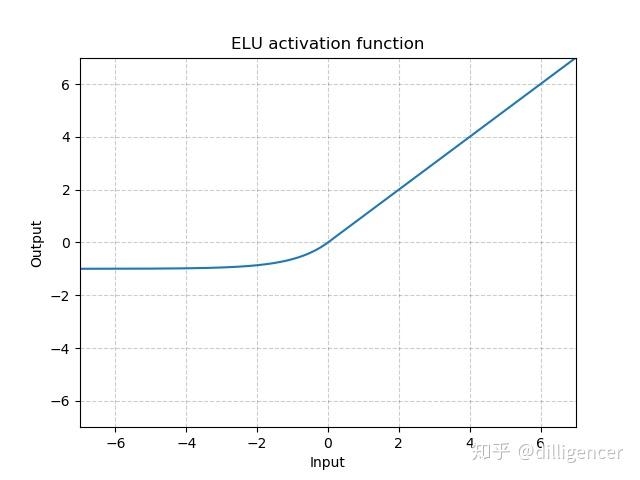
`torch.nn.ELU`(alpha=1.0,inplace=False)

def elu(x,alpha=1.0,inplace=False):
    return max(0,x)+min(0,alpha∗(exp(x)−1))

α是超参数，默认为1.0

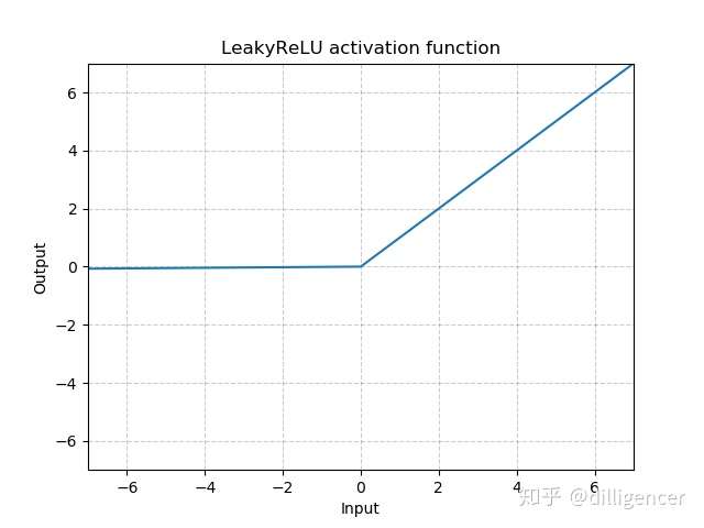
`torch.nn.LeakyReLU`(negative_slope=0.01,inplace=False)

def LeakyReLU(x,negative_slope=0.01,inplace=False):
    return max(0,x)+negative_slope∗min(0,x)

其中 negative_slope是超参数，控制x为负数时斜率的角度，默认为1e-2

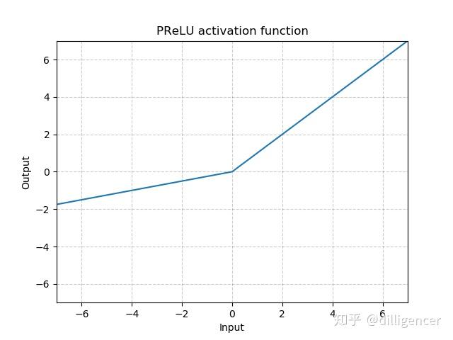
`torch.nn.PReLU`(num_parameters=1,init=0.25)

def PReLU(x,num_parameters=1,init=0.25):
    return max(0,x)+init∗min(0,x)

其中a 是一个可学习的参数，当不带参数调用时，即nn.PReLU()，在所有的输入通道上使用同一个a，当带参数调用时，即nn.PReLU(nChannels)，在每一个通道上学习一个单独的a。

注意：当为了获得好的performance学习一个a时，不要使用weight decay。

num_parameters：要学习的a的个数，默认1

init：a的初始值，默认0.25

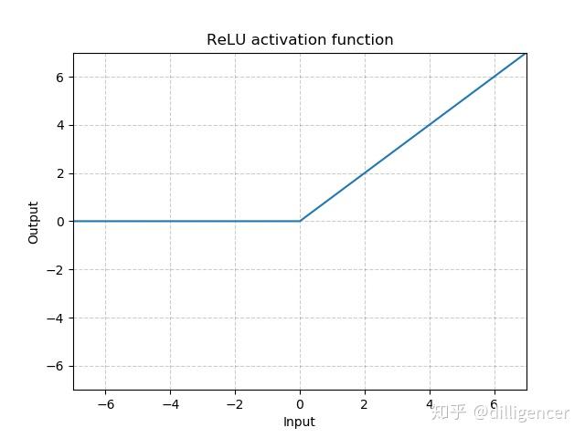
`torch.nn.ReLU`(inplace=False)

CNN中最常用ReLu。

def ReLU(x,inplace=False):
    return max(0,x)

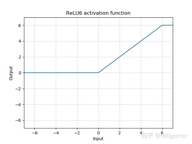
`torch.nn.ReLU6`(inplace=False)

def ReLU6(x,inplace=False):
    return min(max(0,x),6)

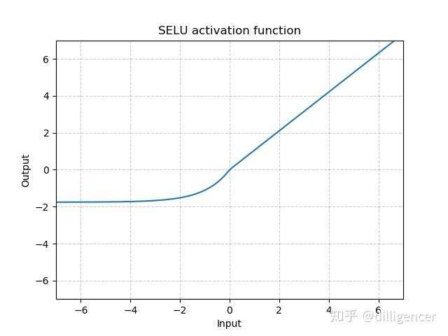
`torch.nn.SELU`(inplace=False)

def SELU(x,inplace=False):
    alpha=1.6732632423543772848170429916717
	scale=1.0507009873554804934193349852946
    return scale∗(max(0,*x*)+min(0,alpha∗(exp(x)−1)))

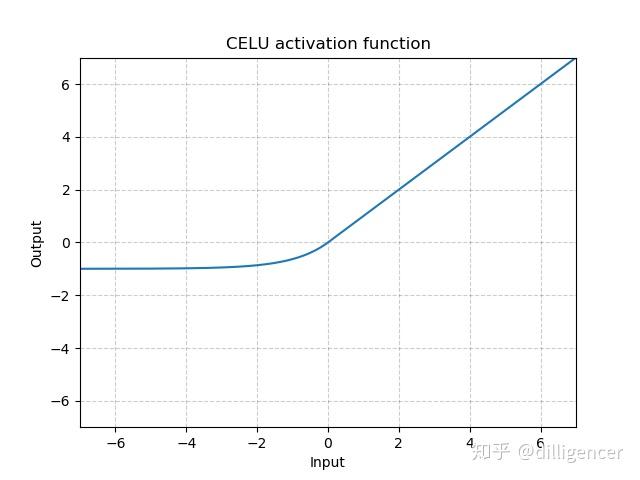
`torch.nn.CELU`(alpha=1.0,inplace=False)

def CELU(x,alpha=1.0,inplace=False):
    return max(0,x)+min(0,alpha∗(exp(x/alpha)−1))

其中α 默认为1.0

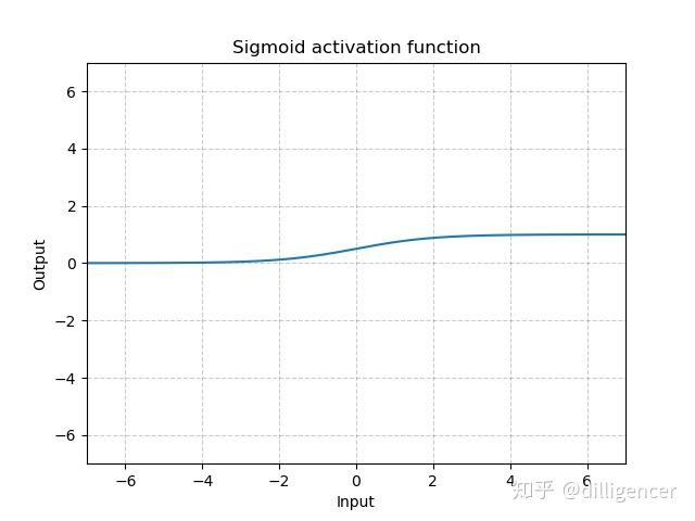
`torch.nn.Sigmoid`

\[ Sigmoid(x)=\frac{1}{1+exp(-x)} \]

def Sigmoid(x):
    return 1/(np.exp(-x)+1)

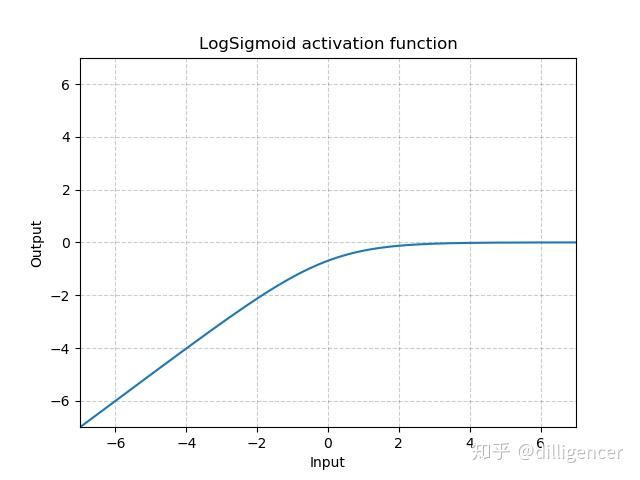
`torch.nn.LogSigmoid`

\[ LogSigmoid(x)=log(\frac{1}{1+exp(-x)}) \]

def LogSigmoid(x):
    return np.log(1/(np.exp(-x)+1))

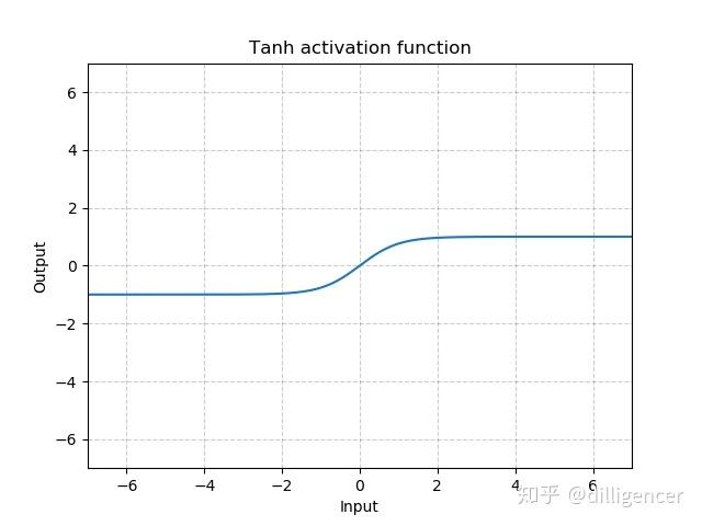
`torch.nn.Tanh`

\[ Tanh(x)=tanh(x)=\frac{e^{x}-e^{-x}}{e^{x}+e^{-x}} \]

def Tanh(x):
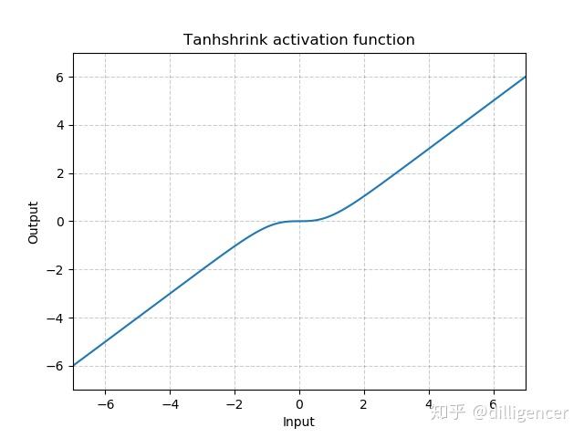
    return (np.exp(x)-np.exp(-x))/(np.exp(x)+np.exp(-x))

`torch.nn.Tanhshrink`

\[ Tanhshrink(x)=x−Tanh(x) \]

def Tanhshrink(x):
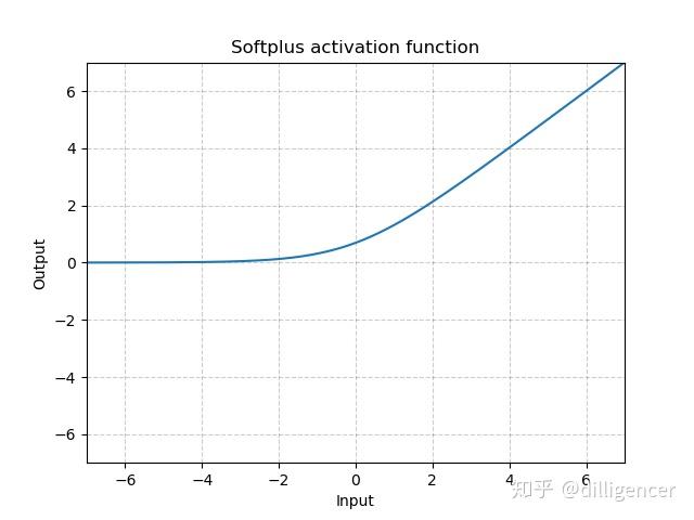
    return x-(np.exp(x)-np.exp(-x))/(np.exp(x)+np.exp(-x))

`torch.nn.Softplus`(beta=1,threshold=20)

\[ Softplus(x)=\frac{1}{\beta}*log(1+exp(\beta*x)) \]

该函数可以看作是ReLu的平滑近似。

def Softplus(x,beta=1,threshold=20):
    return np.log(1+np.exp(beta*x))/beta

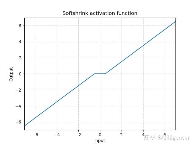
`torch.nn.Softshrink`(lambd=0.5)

\[ SoftShrinkage(x) = \left\{ \begin{array}{ll} x-\lambda, & \textrm{if $x>\lambda$}\\ x+\lambda, & \textrm{if $x<-\lambda$}\\ 0, & \textrm{otherwise} \end{array} \right. \]

λ的值默认设置为0.5

def Softshrink(x,lambd=0.5):
    if x>lambd:return x-lambd
    elif x<-lambd:return x+lambd
    else:return 0

nn.Softmax

\[ Softmax(x_i)=\frac{exp(x_i)}{∑_jexp(x_j)} \]

m = nn.Softmax(dim=1)
input = torch.randn(2, 3)
output = m(input)

参考资料

Pytorch激活函数及优缺点比较

PyTorch快速入门教程二（线性回归以及logistic回归）

Pytorch全连接网络

pytorch系列7 -----nn.Sequential讲解

Pytorch与深度学习自查手册3-模型定义

定义神经网络

权重初始化

方法1：net.apply(weights_init)

方法2：在网络初始化的时候进行参数初始化

常用的操作

利用nn.Parameter()设计新的层

nn.Flatten

nn.Sequential

常用的层

全连接层nn.Linear()

torch.nn.Dropout

卷积torch.nn.ConvNd()

池化

最大池化torch.nn.MaxPoolNd()

均值池化torch.nn.AvgPoolNd()

反池化

最大值反池化nn.MaxUnpool2d()

组合池化

正则化层

BatchNorm

LayerNorm

InstanceNorm

GroupNorm

激活函数

torch.nn.GELU

torch.nn.ELU(alpha=1.0,inplace=False)

torch.nn.LeakyReLU(negative_slope=0.01,inplace=False)

torch.nn.PReLU(num_parameters=1,init=0.25)

torch.nn.ReLU(inplace=False)

torch.nn.ReLU6(inplace=False)

torch.nn.SELU(inplace=False)

torch.nn.CELU(alpha=1.0,inplace=False)

torch.nn.Sigmoid

torch.nn.LogSigmoid

torch.nn.Tanh

torch.nn.Tanhshrink

torch.nn.Softplus(beta=1,threshold=20)

torch.nn.Softshrink(lambd=0.5)